ISLE 6 workshop: Replication and Reproducibility in English Corpus Linguistics
Martin Schweinberger (UQ, UiT)
2022-09-13

Introduction

This document contains the materials for the reproducibility part of the workshop Replication and Reproducibility in English Corpus Linguistics organized by Martin Schweinberger and Joseph Flanagan at the 6th meeting of the International Society for the Linguistics of English (ISLE6) hosted by the University of Eastern Finland. The workshop is held on June 2, 2021; ISLE6 takes place between June 2 and June 5, 2021.
The workshop introduces basic data management techniques, version control measures, and issues relating to reproducible research. The entire R markdown document for this workshop session can be downloaded here. The GitHub repo for this workshop can be found here. A more detailed introduction to data management, version control, and reproducible research practices can be found on the website of the Language Technology and Data Analysis Laboratory (LADAL). Some of the contents of this tutorial build on Amanda Miotto’s Reproducible Reseach Things.
When working with any sort of data on your computer, issues relating to organizing files and folders, managing data and projects, avoiding data loss, and efficient work flows are essential. The idea behind this workshop section is to address this issue and to provide advice on how to handle data and creating efficient workflows that will help you (and your team) in your research.
This part of the workshop consists out of 2 parts:
Data Management
This part of the workshop focuses on general principles that help to organize your data and help maintain efficient workflows.Optimizing workflows in RStudio
This part of the workshop focuses on how to optimize your workflows in RStudio and how to create reproducible and robust data processing and analysis chains.
As this workshop is introductory, we will only highlight the most basic ways and tools that you can use to improve your workflows and make them reproducible. We cannot focus on any of the tools in great detail as we want to cover as much ground as possible.
1 Data Management
This section introduces some basic concepts and provides useful tips for managing your research data.
Folder structure
There are various ways in which you can organize your folders. All of these ways to organize your folders have different advantages and problems but they all have in common that they rely on a tree-structure - more general folders contain more specialized ones. For example, if you want to find any file with as few clicks as possible, an alphabetical folder structure would be a good solution. Organized in this way, everything that starts with a certain letter will be stored by its initial letter (e.g. everything starting with a t such as travel under T or everything related to your courses under C). However, organizing your data alphabetically is not intuitive and completely unrelated topics will be located in the same folder.
A more common and intuitive way to organize your data is to separate your data into meaningful aspects of your life such as Work (containing, e.g., teaching and research), Living (including rent, finances, and insurances), and Media (including Movies, Music, and Audiobooks).
Naming conventions
A File Naming Convention (FNC) is a framework or protocol if you like for naming your files in a way that describes what files contain and importantly, how they relate to other files. It is essential prior to collecting data to establish an agreed FNC.
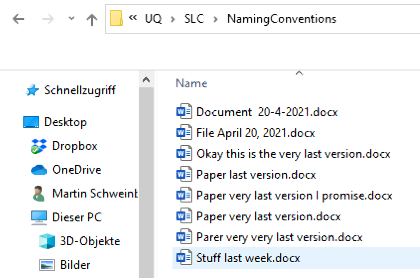
Folders (as well as files) should be labeled in a meaningful way. This means that you avoid names like Stuff or Document for folders and doc2 or homework for files.
Naming files consistently, logically and in a predictable manner will prevent against unorganized files, misplaced or lost data. It could also prevent possible backlogs or project delays. A file naming convention will ensure files are:
Easier to process - All team members won’t have to over think the file naming process
Easier to facilitate access, retrieval and storage of files
Easier to browse through files saving time and effort
Harder to lose!
Check for obsolete or duplicate records
The University of Edinburgh has a comprehensive and easy to follow list (with examples and explanations) of 13 Rules for file naming conventions. You can also use the recommendations of the
Australian National Data Services (ANDS) guide of file wrangling. Some of the suggestions are summarized below.
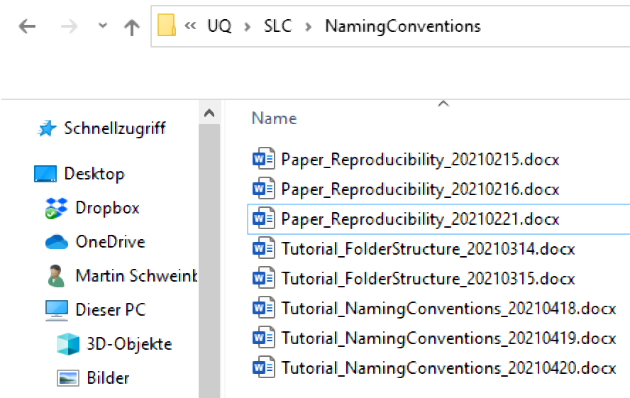
Like the different conventions for folders, there are different conventions for files. As a general rule, any special character symbols, such as +, !, ", -, ., ö, ü, ä, %, &, (, ), [, ], &, $, =, ?, ’, #, or / but also including white spaces, should be avoided (while _ is also a special character, it is still common practice to include them in file names for readability). One reason for this is that you will may encounter problems when sharing files if you avoid white spaces and special characters. Also, some software applications automatically replace or collapse white spaces. A common practice to avoid this issue is to capitalize initial letters in file names which allows you avoid white spaces. An example would be TutorialIntroComputerSkills or Tutorial_IntroComputerSkills.
When you want to include time-stamps in file names, the best way to do this is to use the YYYYMMDD format (rather than DDMMYYYY or even D.M.YY). The reason is that if dates are added this way, the files can be easily sorted in ascending or descending order. To elaborate on the examples shown before, we may use TutorialIntroComputerSkills20200413 or Tutorial_IntroComputerSkills_20200413
Documentation and the Bus Factor
Documentation is the idea of documenting your work so that outsiders (or yourself after a long time) can understand what you did and how you did it. As a general rule, you should document where to find what as if you informed someone else how to find stuff on your computer.
Documentation can include where your results and data are saved but it can also go far beyond this. Documentation does not have to be complex and it can come in different forms, depending on your needs and your work. Documenting what you do can also include photos, word documents with descriptions, or websites that detail how you work.
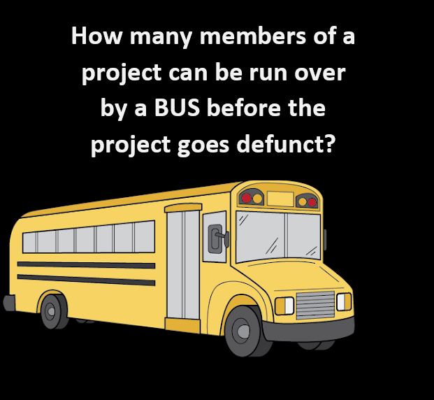
The idea behind documentation is to keep a log of the contents of folders so that you at a later point in time or someone else can continue your work in case you or someone else is run over by a bus (hence the Bus Factor).
In fact, documentation is all about changing the Bus Factor - how many people on a project would need to be hit by a bus to make a project fail. Many times, projects can have a bus factor of one. Adding documentation means when someone goes on leave, needs to take leave suddenly or finishes their study, their work is preserved for your project.
If you work in a collaborative project, it is especially useful to have a log of where one can find relevant information and who to ask for help with what. Ideally you want to document anything that someone coming on board would need to know. Thus, if you have not created a log for on-boarding, the perfect person to create a log would be the last person who joined the project. Although there is no fixed rule, it is recommendable to store the log either as a ReadMe document or in a ReadMe folder on the top level of the project.
Keep copies
Keeping a copy of all your data (working, raw and completed) in the cloud is incredibly important. This ensures that if you have a computer failure, accidentally delete your data or your data is corrupted, your research is recoverable and restorable.
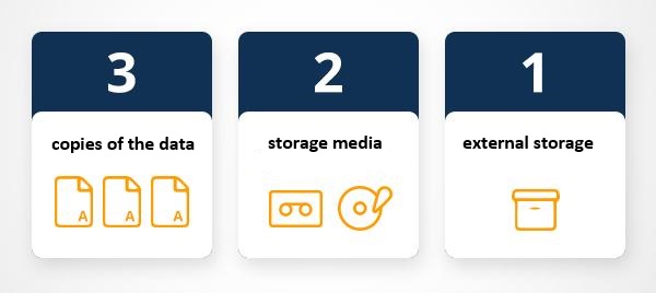
The 3-2-1 backup rule
Try to have at least three copies of your project that are in different locations. The rule is: keep at least three (3) copies of your data, and store backup-copies on two (2) different storage media , with one (1) of them located offsite. Although this is just a personal preference, I always safe my projects
on my personal notebook
on at least one additional hard drive (that you keep in a secure location)
in an online repository (for example, UQ’s Research Data Management system (RDM) OneDrive, MyDrive, GitHub, or GitLab)
Using online repositories ensures that you do not lose any data in case your computer crashes (or in case you spill lemonade over it - don’t ask…) but it comes at the cost that your data can be more accessible to (criminal or other) third parties. Thus, if you are dealing with sensitive data, I suggest to store it on an additional external hard drive and do not keep cloud-based back-ups. If you trust tech companies with your data (or think that they are not interested in stealing your data), cloud-based solutions such as OneDrive, Google’s MyDrive, or Dropbox are ideal and easy to use options (however, UQ’s RDM is a safer option).
The UQ library also offers additional information on complying with ARC and NHMRC data management plan requirements and that UQ RDM meets these requirements for sensitive data (see here).
Avoid duplicates

Many of the files on our computers have several duplicates or copies on the same machine. Optimally, each file should only be stored once (on one machine). Thus, to minimize the superfluous files on your computer, we can delete any duplicates of files.
You can, of course, do that manually but a better way to do this is to use programs that detect files that are identical in name, file size, and date of creation. One of these programs is the Douplicate Cleaner. A tutorial on how to use it can be found here.
How to organize projects
This section focuses on how to organize your projects and how to use your computer in doing so.
Project folder design
Having a standard folder structure can keep your files neat and tidy and save you time looking for data. It can also help if you are sharing files with colleagues and having a standard place to put working data and documentation.
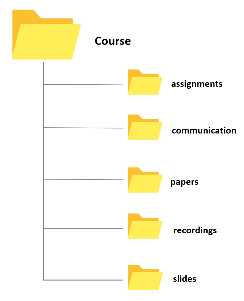
Store your projects in a separate folder. For instance, if you are creating a folder for a research project, create the project folder within a separate project folder that is within a research folder. If you are creating a folder for a course, create the course folder within a courses folder within a teaching folder, etc.
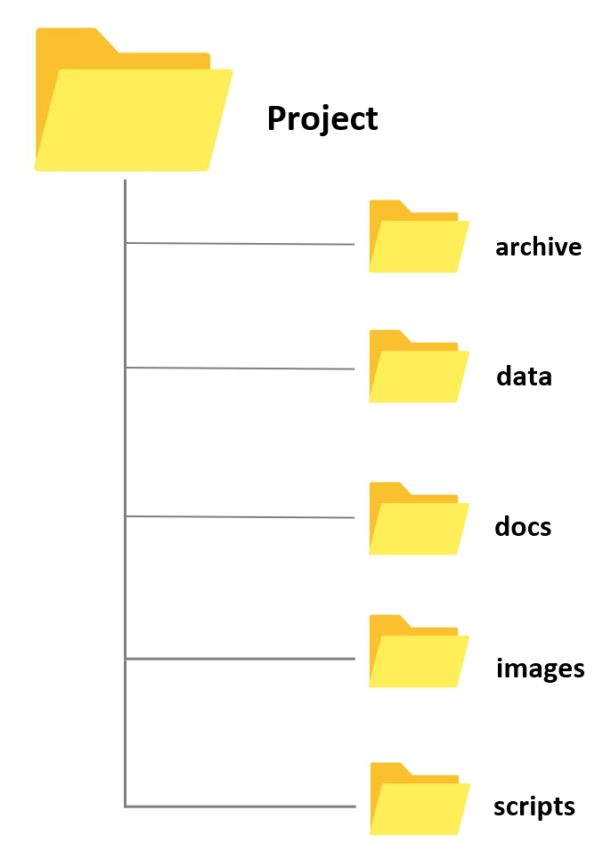
Whenever you create a folder for a new project, try to have a set of standard folders. For example, when I create research project folders, I always have folders called archive, data, docs, and images. When I create course folders, I always have folders called slides, assignments, exam, studentmaterials, and correspondence. However, you are, of course, free to modify and come up or create your own basic project design. Also, by prefixing the folder names with numbers, you can force your files to be ordered by the steps in your workflow.
- Having different sub folders allows you to avoid having too many files and many different file types in a single folder. Folders with many different files and file types tend to be chaotic and can be confusing. In addition, I have one ReadMe file on the highest level (which only contains folders except for this one single file) in which I describe very briefly what the folder is about and which folders contain which documents as well as some basic information about the folder (e.g. why and when I created it). This ReadMe file is intended both for me as a reminder what this folder is about and what it contains but also for others in case I hand the project over to someone else who continues the project or for someone who takes over my course and needs to use my materials.
If you work in a team or share files and folders regularly, it makes sense to develop a logical structure for your team, you need to consider the following points:
Check to make sure there are no pre-existing folder structure agreements
Name folders appropriately and in a meaningful manner. Don’t use staff names and consider using the type of work
Consistency - make sure you use the agreed structure/hierarchy
Structure folders hierarchically - start with a limited number of folders for the broader topics, and then create more specific folders within these
Separate ongoing and completed work - as you start to create lots of folders and files, it is a good idea to start thinking about separating your older documents from those you are currently working on
Backup – ensure folders and files are backed up and retrievable in the event of a disaster. UQ like most universities, have safe storage solutions.
Clean up folders and files post project.
Data as publications
More recently, regarding data as a form of publications has gain a lot of traction. This has the advantage that it rewards researchers who put a lot of work into compiling data and it has created an incentive for making data available, e.g. for replication. The UQ RDM and UQ eSpace can help with the process of publishing a dataset.

There are many platforms where data can be published and made available in a sustainable manner. Below are listed just some options that are recommendable:
UQ Research Data Manager
The UQ Research Data Manager (RDM) system is a robust, world-leading system designed and developed here at UQ. The UQ RDM provides the UQ research community with a collaborative, safe and secure large-scale storage facility to practice good stewardship of research data. The European Commission report “Turning FAIR into Reality” cites UQ’s RDM as an exemplar of, and approach to, good research data management practice. The disadvantage of RDM is that it is not available to everybody but restricted to UQ staff, affiliates, and collaborators.
Open Science Foundation
The Open Science Foundation (OSF) is a free, global open platform to support your research and enable collaboration.
TROLLing
TROLLing | DataverseNO (The Tromsø Repository of Language and Linguistics) is a repository of data, code, and other related materials used in linguistic research. The repository is open access, which means that all information is available to everyone. All postings are accompanied by searchable metadata that identify the researchers, the languages and linguistic phenomena involved, the statistical methods applied, and scholarly publications based on the data (where relevant).
Git
GitHub offers the distributed version control using Git. While GitHub is not designed to host research data, it can be used to share small collections of research data and make them available to the public. The size restrictions and the fact that GitHub is a commercial enterprise owned by Microsoft are disadvantages of this as well as alternative, but comparable platforms such as GitLab.
2 Optimizing workflows in RStudio
Most researchers in the language science are familiar to R to some extend. However, while workshops on how to perform particular tasks in R, such as how to do statistical analyses in R, are becoming more widespread, there rarely exist any workshops on how to work in R.

By working in R, I am referring to issues relating to reproducible and effective work flows and session management but also to formatting conventions for R code. The following sections will provide some guidance on how to optimize your work flows and how to make your research practices more transparent, efficient, and reproducible.
Installing R and RStudio
You have NOT yet installed R on your computer?
You have NOT yet installed RStudio on your computer?
- Click here for downloading and installing RStudio.
You can find a more elaborate explanation of how to download and install R and RStudio here that was created by the UQ library.
Rproj
If you’re using RStudio, you have the option of creating a new R project. A project is simply a working directory designated with a .RProj file. When you open a project (using File/Open Project in RStudio or by double–clicking on the .RProj file outside of R), the working directory will automatically be set to the directory that the .RProj file is located in. Using Rprojects makes working in and with R much easier and you can always return exactly to where you left of when you closed the Rproject.
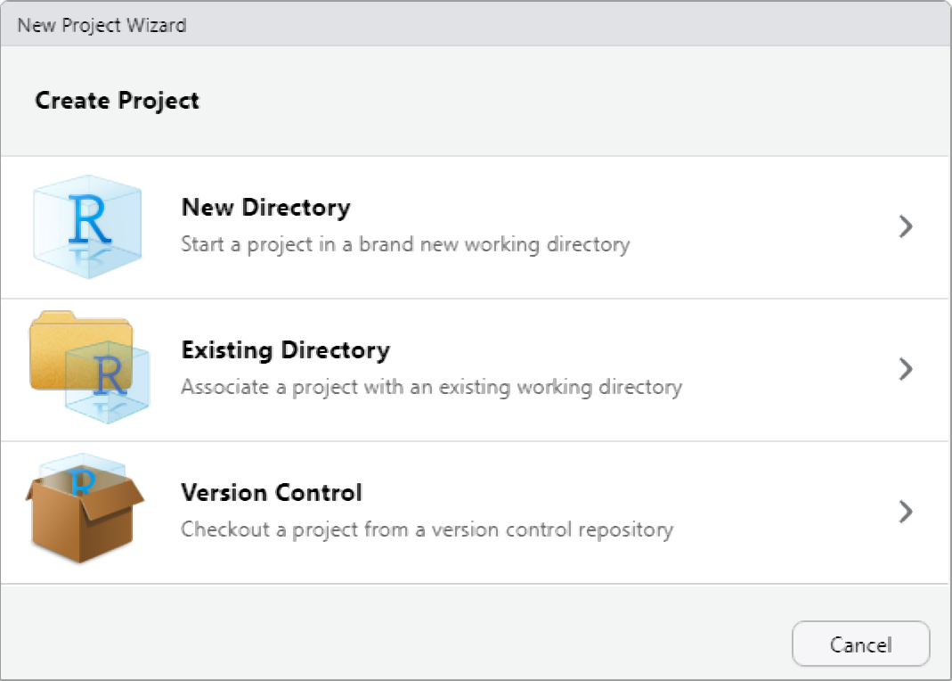
I recommend creating a new R Project whenever you are starting a new research project. Once you’ve created a new R project, you should immediately create folders in the directory which will contain your R code, data files, notes, and other material relevant to your project (you can do this outside of R on your computer, or in the Files window of RStudio). For example, you could create a folder called scripts that contains all of your R code (the scripts), a folder called data that contains all your data, a folder called images for your visualizations, etc.
Before working with Rprojects, I set my working directories with setwd() but this is not optimal because it takes an absolute file path as an input then sets it as the current working directory of the R process. However, this makes scripts break easily and it makes it more difficult to share my analyses and projects with others. Hence, the setwd() approach makes it very difficult to share work and make it transparent and reproducible.
Solving dependency issues: renv
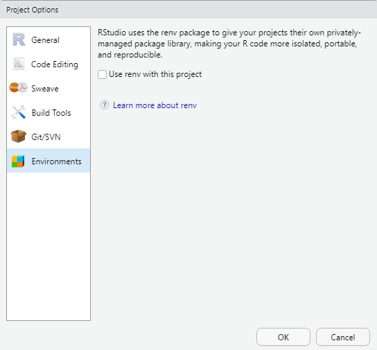
The renv package is a new way to make Rprojects independent and thus to remove outside dependencies from Rprojects. The renv package creates a new library within your project so that your Rproject is independent of your personal library and when you share your project, you automatically also share the packages that you have used. The idea behind renv is to be a robust, stable replacement for the packrat package which was rather unsatisfactory to work with (speaking from experience here).
I have used renv and, while it took some time to generate the local library on first use, it was very easy to use, did not cause any issues and is overall very recommendable to get rid of outside dependencies and thus make Rprojects easier to share for transparency and reproducibility.
Underlying the philosophy of renv is that all existing work flows should just work as they did before – renv helps to isolate your project’s R dependencies (like package versioning).
You can get more information about renv and how it works, as well as how you can use it here.
Version Control with Git
Getting started with Git
To connect your Rproject with GitHub, you need to have Git installed (if you have not yet downloaded and installed Git, simply search for download git in your favorite search engine and follow the instructions) and you need to have a GitHub account. If you do not have a GitHub account, here is a video tutorial showing how you can do this. If you have trouble with this, you can also check out Happy Git and GitHub for the useR at happygitwithr.com.
Just as a word of warning: when I set up my connection to Git and GitHUb things worked very differently, so things may be a bit different on your machine. In any case, I highly recommend this YouTube tutorial which shows how to connect to Git and GitHub using the usethis package or this, slightly older, YouTube tutorial on how to get going with Git and GitHub when working with RStudio.
Old school
While many people use the usethis package to connect RStudio to GitHub, I still use a somewhat old school way to connect my projects with GitHub. I have decided to show you how to connect RStudio to GitHub using this method, as I actually think it is easier once you have installed Git and created a gitHub account.
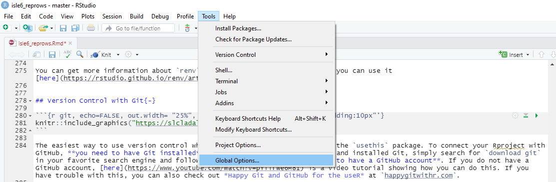
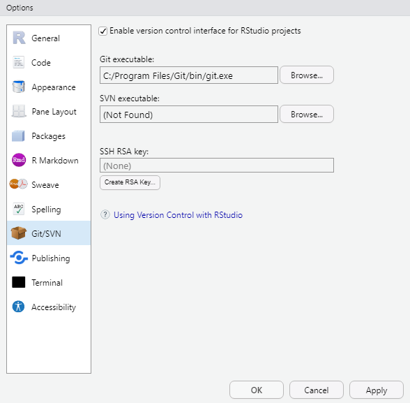
Before you can use Git with R, you need to tell RStudio that you want to use Git. To do this, go to Tools, then Global Options and then to Git/SVN and make sure that the box labeled Enable version control interface for RStudio projects. is checked. You need to then browse to the Git executable file (for Window’s users this is called the Git.exe file).
Now, we can connect our project to Git (not to GitHub yet). To do this, go to Tools, then to Project Options... and in the Git/SVN tab, change Version Control System to Git (from None). Once you have accepted these changes, a new tab called Git appears in the upper right pane of RStudio (you may need to / be asked to restart RStudio at this point). You can now commit files and changes in files to Git.
To commit files, go to the Git tab and check the boxes next to the files you would like to commit (this is called staging; meaning that these files are now ready to be committed). Then, click on Commit and enter a message in the pop-up window that appears. Finally, click on the commit button under the message window.
Connecting your Rproj with GitHub
To connect your Rproject and GitHub, we go to our GitHub page and create a new GitHub repository (repo) that we call test (or whatever you want to call your repository). To create a new repository on GitHub, simply click on New Repository after you have clicked on the New icon. I recommend that you check Add a Readme in which you can describe what the repo contains, but you do not have to do this.
Once you have created a new GitHub repo, we need to connect this repo to our computer. To do this, we need to clone the repo which we do by clicking on the green Code icon. When you click on the green Code icon, a dropdown menu appears and you copy the url in the section clone with HTTPS.
Then, we go to the Terminal (in-between Console and Jobs) and we include the path we got from the git repository after the command git remote add origin. We then use the command git branch -M main (to merge a master and a main branch) and then, finally, push our files into the remote GitHub repo by using the command git push -u origin main.
# initiate the upstream tracking of the project on the GitHub repo
git remote add origin https://github.com/MartinSchweinberger/test.git
# set main as main branch (rather than master)
git branch -M main
# push content to main
git push -u origin main
We can then commit changes and push them to the remote GitHub repo.
You can then go to your GitHub repo and check if the documents that we pushed are now in the remote repo.
From now on, you can simply commit all changes that you make to the GitHub repo associated with that Rproject. Other projects can, of course, be connected and push to other GitHub repos.
Solving path issues: here
The goal of the here package is to enable easy file referencing in project-oriented workflows. In contrast to using setwd(), which is fragile and dependent on the way you organize your files, here uses the top-level directory of a project to easily build paths to files.
This makes your projects more robust as the paths will still work if you put your project into another location or on another computer. Also, moving between Mac and Windows (which would require different kind of path specifications) is no longer an issue with the here package.
# define path
example_path_full <- "D:\\Uni\\Konferenzen\\ISLE\\ISLE_2021\\isle6_reprows/repro.Rmd"
# show path
example_path_full
## [1] "D:\\Uni\\Konferenzen\\ISLE\\ISLE_2021\\isle6_reprows/repro.Rmd"With the here package, the path starts in folder where the Rproj file is. As the Rmd file is in the same folder, we only need to specify the Rmd file and the here package will add the rest.
# load package
library(here)
# define path using here
example_path_here <- here::here("repro.Rmd")
#show path
example_path_here
## [1] "/home/sam/programming/SLCLADAL.github.io/repro.Rmd"Reproducible randomness: set.seed
The set.seed function in R sets the seed of R‘s random number generator, which is useful for creating simulations or random objects that can be reproduced. This means that when you call a function that uses some form of randomness (e.g. when using random forests), using the set.seed function allows you to replicate results.
Below is an example of what I mean. First, we generate a random sample from a vector.
numbers <- 1:10
randomnumbers1 <- sample(numbers, 10)
randomnumbers1
## [1] 3 6 1 5 8 7 4 10 2 9We now draw another random sample using the same sample call.
randomnumbers2 <- sample(numbers, 10)
randomnumbers2
## [1] 7 5 3 10 8 4 9 2 6 1As you can see, we now have a different string of numbers although we used the same call. However, when we set the seed and then generate a string of numbers as show below, we create a reproducible random sample.
set.seed(123)
randomnumbers3 <- sample(numbers, 10)
randomnumbers3
## [1] 3 10 2 8 6 9 1 7 5 4To show that we can reproduce this sample, we call the same seed and then generate another random sample which will be the same as the previous one because we have set the seed.
set.seed(123)
randomnumbers4 <- sample(numbers, 10)
randomnumbers4
## [1] 3 10 2 8 6 9 1 7 5 4Citation & Session Info
Schweinberger, Martin. 2022. ISLE 6 workshop: Replication and Reproducibility in English Corpus Linguistics. Brisbane: The University of Queensland. url: https://slcladal.github.io/isle6_reprows.html (Version 2022.09.13).
@manual{schweinberger2022reprows,
  author = {Schweinberger, Martin},
  title = {ISLE 6 workshop: Replication and Reproducibility in English Corpus Linguistics},
  note = {https://slcladal.github.io/isle6_reprows.html},
  year = {2022},
  organization = {The University of Queensland, School of Languages and Cultures},
  address = {Brisbane},
  edition = {2022.09.13}
}sessionInfo()## R version 4.2.1 (2022-06-23)
## Platform: x86_64-pc-linux-gnu (64-bit)
## Running under: Ubuntu 22.04.1 LTS
##
## Matrix products: default
## BLAS: /usr/lib/x86_64-linux-gnu/blas/libblas.so.3.10.0
## LAPACK: /usr/lib/x86_64-linux-gnu/lapack/liblapack.so.3.10.0
##
## locale:
## [1] LC_CTYPE=en_AU.UTF-8 LC_NUMERIC=C
## [3] LC_TIME=en_AU.UTF-8 LC_COLLATE=en_AU.UTF-8
## [5] LC_MONETARY=en_AU.UTF-8 LC_MESSAGES=en_AU.UTF-8
## [7] LC_PAPER=en_AU.UTF-8 LC_NAME=C
## [9] LC_ADDRESS=C LC_TELEPHONE=C
## [11] LC_MEASUREMENT=en_AU.UTF-8 LC_IDENTIFICATION=C
##
## attached base packages:
## [1] stats graphics grDevices datasets utils methods base
##
## other attached packages:
## [1] here_1.0.1 DT_0.24
##
## loaded via a namespace (and not attached):
## [1] rprojroot_2.0.3 digest_0.6.29 R6_2.5.1 jsonlite_1.8.0
## [5] magrittr_2.0.3 evaluate_0.15 highr_0.9 stringi_1.7.8
## [9] rlang_1.0.4 cli_3.3.0 renv_0.15.4 jquerylib_0.1.4
## [13] bslib_0.3.1 rmarkdown_2.14 tools_4.2.1 stringr_1.4.0
## [17] htmlwidgets_1.5.4 xfun_0.31 yaml_2.3.5 fastmap_1.1.0
## [21] compiler_4.2.1 htmltools_0.5.2 knitr_1.39 sass_0.4.1